Historical Timeline of Derivatives

Posted on 20222022 by M. Humayun Kabir

...... Nobody can hope to understand the economic phenomena of any, including the present, epoch, who has not an adequate command of historical facts and an adequate amount of historical sense or of what might be described as historical experience. ........ the historical report cannot be purely economic but must inevitably reflect also "institutional" facts that are not purely economic: therefore it affords the best method for understanding how economic and non-economic facts are related to one another and how the various social sciences should be related to one another. ....... the fact that most of the fundamental errors currently committed in economic analysis are due to lack of historical experience more often than to any other shortcoming of the economist's equipment. History must of course be understood to include fields that have acquired different names as a consequence of specialization, such as prehistoric events and ethnology (anthropology) - Joseph A. Schumpeter, History of Economic Analysis, Elizabeth Boody Schumpeter, ed. (New York: Oxford University Press, 1954), pp. 12-13.

8000 BCE

In Sumer, located in the Tigris and Euphrates river region, a unique accounting method was developed using clay tokens in 8000 B.C. The clay tokens were baked into a spherical sort of envelope and used as a promise to a counterparty to deliver a quantity of goods by a certain date. Based on the timeframe imprinted into the envelope vessel and the tokens themselves, sellers promised to deliver the assets. This exchange essentially functioned as a sort of forward contract, which was settled once the seller delivered their goods by the date baked onto the token.

1750 BCE

“If any one owe a debt for a loan, and a storm prostrates the grain, or the harvest fail, or the grain does not grow for lack of water; in that year he need not give his creditor any grain, he washes his debt-tablet in water and pays no rent for the year.” - 48th law from the Code of Hammurabi.

Hammurabi, who was the king of Babylon devised a code to ensure that farmers having loans on their houses were not required to pay annual interest in the form of grain in the event of crop failure. In such a scenario, farmers' right not to pay interests is similar to what we now-a-days call put options.

1600 CE

Forward and option contracts on tulip bulbs flourish in Holland. Tulip bulb prices collapse in the winter of 1637,
causing significant contract default.

350 BCE

Options to rent olive presses are described in Aristotle’s Politics.

1848 CE

Chicago Board of Trade (CBT) is formed on April 3, 1848, to provide a centralized marketplace for cash and forward transactions in grains.

1865 CE

CBT revamps forward markets by introducing futures contracts on agricultural commodities. These new contracts were standardized contracts in terms of quality, quantity, time & place of delivery, and involved the use of a clearinghouse and a system of margining.

1874 CE

Chicago Produce Exchange (CPE) is formed to trade futures on butter, eggs, poultry, and other perishable products.

1878 CE

London Corn Trade Association introduces the ﬁrst futures contract in the United Kingdom.

1882 CE

Coffee Exchange (CE) is formed by a group of coffee merchants to trade futures on coffee.

1898 CE

Butter and egg dealers withdraw from the CPE to form the Chicago Butter and Egg Board (CBEB).

1904 CE

Winnipeg Commodity Exchange (WCE) introduces ﬁrst commodity (oat) futures contracts in Canada.

1933 CE

Commodity Exchange (COMEX) is formed and introduces the ﬁrst futures contract on a non-agricultural commodity — silver.

1952 CE

London Metal Exchange (LME) lists the ﬁrst metal (lead) futures contract in October in the U.K.

1961 CE

Chicago Mercantile Exchange (CME) introduces the ﬁrst futures contract on livestock - frozen pork bellies.

1972 CE

CME introduces the ﬁrst futures contract written on a ﬁnancial instrument, which was on foreign currencies.

1973 CE

CBT organizes the Chicago Board Options Exchange (CBOE) for the purpose of trading call options on 16
New York Stock Exchange (NYSE) common stocks.

1975 CE

CBT introduces ﬁrst interest rate futures contracts — Government National Mortgage Association (GNMA) futures. In the same year in January American Stock Exchange (AMEX) launches call options on stocks.

1977 CE

CBOE and AMEX listed for the ﬁrst time put options on common stocks are. CBT also launched Treasury bond futures contracts.

1980 CE

The first over-the-counter (OTC) Treasury bond option takes place.

1981 CE

Interest rate swap transaction takes place for the first time over-the-counter (OTC). CME introduces the Eurodollar futures, which is the ﬁrst cash settlement futures contract.

1991 CE

The notional amount of OTC derivatives trading surpasses exchange-traded derivatives.

1992 CE

Credit derivative contracts begin trading in the OTC market.

2004 CE

CBOE launches futures contract written on CBOE Market Volatility Index (VIX).

Why is there a Derivative Market?

Posted on 2022 by M. Humayun Kabir

WHY IS THERE A DERIVATIVE MARKET?

Why does someone take a long or short position in the derivative contract rather than buying and selling on the spot? The answer to this question, in fact, is the answer to the question: why does the derivative market exist?

First, a derivative contract allows you to delay the purchase or sale of an underlying asset. Rather than buying on the spot, you can buy on some specified future date depending on your expectations about the price movements. If you expect the price to go down in the future, enter into a contract to buy later. You enter into a contract when you expect the price to go up.

Second, when you enter into a derivative contract, you do not pay anything at the initiation of the contract. However, for some contracts like options, you must pay upfront to enter into contracts; but that is far cheaper than the underlying asset (more on options later).

Third, you can either limit or eliminate the downside risk or take advantage of the upside potential, or both at the same time.

Fourth, derivatives make it possible to transfer risk. The underlying of a derivative contract bears several risks. The shares of a firm are associated with the risk of prices going up or down (price risk). A derivative on stock transfers the risk from the seller to the buyer or the seller to the buyer. A bond bears with it risks associated with the interest rate, credit, or currency (if the bond is issued in a different currency than the domestic currency). A derivative instrument written on a bond transfers interest rate risks (interest rate derivatives) or credit risk (credit default swap).

Transferring risk leads to hedging, which is one of the most important aspects of derivatives. If you currently hold 100 shares of Apple Inc., your concern is the risk of prices going down. To offset the risk, you can enter into a derivative contract written on Apple Inc. stock to sell the shares at a price that ensures profits. Here you lock in some prize or profit in the future. By holding the shares, you are faced with some risk exposure. This risk exposure is offset by entering into the derivative contract. If you do not hold any Apple Inc. shares, you don't have any risk exposure to offset.

Types of Derivatives markets & Instruments

Posted on 2022 by M. Humayun Kabir

TYPES OF DERIVATIVE MARKETS

Broadly, there are two types of derivatives markets:

Over-the-counter market (OTC): In the OTC market, the derivatives contracts are negotiated privately between parties. There might be a middle party who facilitates such negotiation for commission. There are no specific or particular contract specifications.
Organized exchange: In organized exchanges, such as Chicago Mercantile Exchange (CME), New York Mercantile Exchange (NYMEX), and Chicago Board Options Exchange (CBOE), the contract specifications for listed derivatives are standardized. Buyers and sellers in such exchanges trade following the rules specified by the change. Order execution through an exchange facilitates transparency, liquidity, and price discovery.

TYPES OF DERIVATIVE INSTRUMENTS

There are many kinds of derivative instruments. Broadly, we can categorize it into the following types:

Forwards: a contractual agreement between two parties over-the-counter to buy or sell a product on a future date at a pre-determined price negotiated today. You do not pay anything upfront.
Futures: a contractual agreement between two parties in an organized exchange to buy or sell a product on a future date at a pre-determined price negotiated today. You do not pay anything upfront, but there is a margin requirement.
Options: a contractual agreement between two parties over-the-counter or in an organized exchange to buy or sell a product on a future date at a pre-determined price negotiated today. You must pay a premium upfront.
Swap: a contractual agreement between two parties over-the-counter to exchange cash flows on a notional principal of an underlying on future dates periodically until maturity.

Long & Short Positions

Posted on 20222022 by M. Humayun Kabir

LONG & SHORT POSITIONS

When someone negotiates a derivative contract to buy the underlying on a future day, he or she is said to have a long position in the contract (example 1). The other side of the contract, the counterparty, is in a short position, Similarly, if you decide to sell something on a future date under the contract your position would be a short position (example 2). The counterparty of the contract would have a long position.

The party in the long position benefits from a derivative transaction if the price of the underlying increases in the future (example 1).
The party in the short position benefits from a derivative transaction if the price of the underlying decreases in the future (example 2).

What is a Derivative?

Posted on 20222022 by M. Humayun Kabir

WHAT IS A DERIVATIVE?

In the spot market, we buy and sell products immediately. In the derivative market, we buy and sell on a future date, but we negotiate contracts today. A derivative is a contractual agreement between two parties to buy or sell a product on a future date at a pre-determined price negotiated today.
The future date is the expiration day of the contract. The contract is valid until its expiration. The product on which the contract is negotiated is called the underlying. The derivative contracts as such are financial products, the underlying of which can be both real or financial assets. In the financial markets, the underlying can be stocks, bonds, foreign currencies, and equity indexes. These are investment assets. In a broader sense, precious metals like gold, silver, copper, and platinum, though they are not financial assets, are considered investment assets. The real assets are commodities like crude oil, heating oil, gas, corn, rice, wheat, cocoa, soybean, sugar, lumber, cotton, hogs, and cattle which can be underlying for the derivative contracts. We call these commodities the consumption assets.

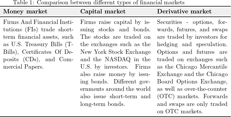
Let's look at the following table to see how the derivative market stands in comparison to the money market and capital market:

Rendered by QuickLaTeX.com

For a better understanding of how a derivative contract works, let's consider the following example:

✓ Example 1

The price of a share of Apple Inc. is $190.92 today. If you want to buy one of Apple Inc. today on the spot, you must pay $190.92. However, today you can negotiate a derivative contract to buy one Apple Inc. share three months from now at $195.50. In this case, the underlying of this derivative contract is one Apple Inc. share, and the contract will expire in three months. You can buy one Apple Inc. share at $195.50 at the expiration date three months from now. This price is called exercise or strike price. In other words, the spot price is $190.92 if you buy today, but the exercise price is $195.50, which you would pay when you buy the share at the expiration of the contract. Under the derivative contract, you postpone your spot purchase today in favor of a future day purchase.

In the above example, if the stock price goes up to $200.00 on the expiration day three months from now, you would not buy the share at the spot price of $200.00 as you can buy cheaper at a price of $195.50 under the derivative agreement. In this case you can save $200.00 - $195.50 = $4.50 per share. Without an agreement, you would have to pay $4.50 more.

If the stock price turns to be $190.50 at expiration, you would have to pay $195.50 under the derivative agreement. In this scenario, you pay $195.50 - $190.50 = $5.00 more per share when compared with spot buying at $190.50. No matter what happens in the market, you would always pay $195.50 under the contract. In other words, you are locked in at a price of $195.50.

Let's consider another example where you want to sell an Apple Inc. share that you own:

✓ Example 2

The price of a share of Apple Inc. is $190.92 today. You may sell one Apple Inc. share today on the spot for $190.92. However, today you can negotiate a derivative contract to sell one Apple Inc. shares three months from now at $195.50, which is the exercise or strike price.

In this example, even if the stock price turns to be $190.50 at expiration, you would be able to sell the share at $195.50 under the derivative agreement. In this scenario, you gain $195.50 - $190.50 = $5.00 more per share when compared with spot selling at $190.50. If the stock price goes up to $200.00 on the expiration day, you still must sell the share at $195.50 under the derivative agreement rather than at the spot price of $200.00. In this case you lose $200.00 - $195.50 = $4.50 per share. In other words, you are locked in at a price of $195.50. No matter what happens in the market, you would always receive $195.50 under the contract.

QUIZ

Let's check your knowledge now:

BEGINNER'S PYTHON

Let's get into Python:

Python: Let's start....

In [94]:

exercise_price = 195.50
Price_at_maturity = 200.00
profit = Price_at_maturity - exercise_price
print("Profit = Price at maturity - Exercise price =", profit)

Profit = Price at maturity - Exercise price = 4.5

Rather than writing variable names in long characters, we can also write easily. # sign is used to indicate that this is a comment, not to be executed as python code.

In [7]:

x = 195.50  #Exercise price
st = 200.00 # Price_at_maturity
profit = st - x
profit

Out[7]:

4.5

If we want to the word "Profit=" before 4.5, we can use the print command:

In [69]:

x = 195.50  #Exercise price
st = 200.00 # Price_at_maturity
profit = st - x
print("Profit =", profit) # The word "Profit" is with capital P, but the variable name profit is in small letter.

Profit = 4.5

Our profit is 4.5, which is in float format (number with decimal places). We can convert float into an integer (no decimal places). This is similar to "round" command: we can also write as follows: profit1 = round(profit). Try yourself. If the number is 4.6, it would be rounded to 5. Any number with decimal more than 0.5 is rounded to next digit.

In [68]:

profit1 = int(profit)   # The results 4.5 is a float, we change it into integer. 
profit1

Out[68]:

In [71]:

profit_round = round(4.6)  # 4.6 is rounded to 5.
profit_round

Out[71]:

In [16]:

profit2 = float(profit)  #Here we revert back to float.
profit

Out[16]:

4.5

Can Python tell me which number is interger, which one float? Yes:

In [17]:

type(4)

Out[17]:

int

In [18]:

type(4.5)

Out[18]:

float

In [20]:

type("Profit") # Here Profit is a string variable.

Out[20]:

str

Let's do some more math calculations:¶

In [75]:

55 - 45 # subtruction

Out[75]:

In [23]:

55 * 5 # multiplication

Out[23]:

In [24]:

55 / 5 #division

Out[24]:

11.0

What does happen if you '//' rather than '/'?¶

In [81]:

57 // 5   # this called floor dividion. Here '//' rounds the result down to the nearest whole number. 
          # Even if we use 58 // 5, we are going to get same result.

Out[81]:

How can we find the value of $5^3$?¶

In [74]:

5 ** 3 # This is 5 to 5 to the power 3.

Out[74]:

Let's consider float again:¶

In [26]:

3/2

Out[26]:

1.5

In [27]:

0.3/0.2

Out[27]:

1.4999999999999998

In [29]:

float(0.3/0.2)

Out[29]:

1.4999999999999998

In [30]:

round(0.3/0.2)

Out[30]:

In [36]:

m = 0.3/0.2
f"The value in two decimal places is {m:.2f}"     # rounds the number to two decimal places

Out[36]:

'The value in two decimal places is 1.50'

In [37]:

n = 6432168151
f"The value of n is {n:,}"   # the value is expressed by grouping in thousands

Out[37]:

'The value of n is 6,432,168,151'

In [39]:

n = 32442.5864
f"The value of n is {n:,.2f}"   # the value is expressed by grouping in thousands and rounded to two decimal places

Out[39]:

'The value of n is 32,442.59'

In [41]:

f"{242392.5065:.2f}"   # 242392.5065 is rounded to two decimal place

Out[41]:

'242392.51'

In [42]:

f"{242392.5065:,.2f}"  # 242392.5065 is rounded to two decimal place and grouped in thousands

Out[42]:

'242,392.51'

In [43]:

f"${242392.5065:,.2f}"   # rounded to two decimal place, grouped in thousands and use currency sign

Out[43]:

'$242,392.51'

Percentages¶

The % sign with 1 before it (1%) displays percentage with one decimal place. It multiplies a number by 100 and displays it in fixed-point format, followed by a percentage sign.¶

In [46]:

n = 0.75
f"{n:.1%}"   # .1% displays the number as a percentage with one decimal place

Out[46]:

'75.0%'

In [47]:

n = 0.75
f"{n:.2%}"   # .2% displays the number as a percentage with two decimal place

Out[47]:

'75.00%'

What about 5 % 2? It will show the reminder of the division. Here '%' is called modulus, which is used to find the remainder in division.¶

In [84]:

5 % 2

Out[84]:

Square root¶

If you want to take square root of some number, then you have import math package. Let's do it:¶

In [92]:

import math
x = 625
y = math.sqrt(x)
print("Square root of x is", y)

Square root of x is 25.0

In [59]:

f"Square root of x is {y:.2f}"

Out[59]:

'Square root of x is 25.20'

We can do the same with numpy package.¶

In [95]:

import numpy as np  # here we have imported numpy "as np"
x = 625
y = np.sqrt(x)      # since we have imported it as np, we can now use np.sqrt(x). Otherwise, we have to write numpy.sqrt(x). 
y

Out[95]:

25.0

In summary:¶

Operator	Description	Syntax
+	Addition	x + y
----------	---------------------	------
–	Subtraction	x – y
----------	---------------------	------
*	Multiplication	x * y
----------	---------------------	------
/	Division (float)	x / y
----------	---------------------	-----
//	Division (floor)	x // y
----------	---------------------	------
%	Modulus: remainder	x % y
----------	---------------------	-----
**	Power	x **y

PRACTICE PYTHON

In the following box you can write codes and evaluate them. Follow the way I have done above.

Tip: Click the arrow on the right side of the cell to evaluate (arrow is shown on mouseover). OR press Shift-ENTER

Compound Interest Rate

Posted on 20222022 by M. Humayun Kabir

Compound Interest Rates

Let's re-state our previous example: if $1,000 is invested for a year at the interest rate of 10% per annum with annual compounding, you are going to receive at the end of the year a return of

$\$1,000 \times 0.10 = \$100$

Your investment earns $100 at the end of the year. The value of your investment at the end of the first year is $1,100. We can write the value of your investment as

$\$1,000 + \$1,000 \times 0.10 = \$1,000(1+0.10) = \$1,100$

If $1,000 is invested for two years at the interest rate of 10% per annum with annual compounding, you are going to receive at the end of the first year a return of

$\$1,000 \times 0.10 = \$100$

The value of your investment is

$\$1,000 + \$1,000 \times 0.10 = \$1,100$

$\$1,000(1+0.10) = \$1,100$

In the second year, you invest $1,100 at 10% for another year. The value of your investment would be

$\$1,100 + \$1,100 \times 0.10 = \$1,210$

$\$1,100(1+0.10) = \$1,210$

Or we can write as follows:

$\$1,100(1+0.10) = \$1,210$

$\$1,000(1+0.10)(1+0.10) = \$1,210$

$\$1,000(1+0.10)^2 = \$1,210$

Now, if you invest $1,210 for the third year at 10%, the value of your investment would be

$\$1,210(1+0.10) = \$1,331$

We can also write the above equation as

$\$1,000(1+0.10)(1+0.10)(1+0.10) = \$1,331$

⇒

$\$1,000(1+0.10)^3 = \$1,331$

We can continue this way for years 4 and 5 with outcomes as follows:

$\$1,000(1+0.10)^4 = \$1,464.10$

$\$1,000(1+0.10)^5 = \$1,610.51$

In this case, your investment of $1,000 earns $610.51 at the end of five years. The value of your investment grows to $1,610.51 rather than $1,500.

In the above example, (1+0.10), (1+0.10)², (1+0.10)³, (1+0.10)⁴, (1+0.10)⁵ show how $1 investment grows every year:

$(1+0.10) = 1.10$

$(1+0.10)^2= 1.21$

$(1+0.10)^3= 1.331$

$(1+0.10)^4= 1.4641$

$(1+0.10)^5= 1.61051$

If you subtract $1 in each equation above, we get the effective interest rate:

$(1+0.10) - 1= 0.10$

$(1+0.10)^2 - 1 = 0.21$

$(1+0.10)^3 - 1 = 0.331$

$(1+0.10)^4 - 1 = 0.4641$

$(1+0.10)^5 -1 = 0.61051$

The effective interest rate when the interest rate compounds annually,

$\left(1+r\right)^t - 1$

Compare the above calculations with the simple interest rate, where interest rates do not compound. It remains 10% without compounding annually. When 10% compounds annually, the effective rate increases from 10% in the first year to 61.051% in the fifth year.

As you can see now that a $1,000 investment at a 10% continuously compounded interest rate can $610.51 as opposed to $500 with a simple interest rate.

Let's $$1,000 = M₀, and (1+0.10)^t = (1+r)^t, then we can write, Future Value, FV_t:

$M_t = M_0(1+r)^t$

In other words, the future value of $1 can be written as (1+r)^t, which is the compound factor.

Let's now consider one year:

When we compound r semi-annually in one year the amount $1 grows to
$\left(1+\frac{r}{2}\right)^2$
When we compound r quarterly in one year the amount $1 grows to
$\left(1+\frac{r}{4}\right)^4$
When we compound r monthly in one year the amount $1 grows to
$\left(1+\frac{r}{12}\right)^{12}$
When we compound r weekly in one year the amount $1 grows to
$\left(1+\frac{r}{52}\right)^{52}$
When we compound r daily in one year the amount $1 grows to
$\left(1+\frac{r}{365}\right)^{365}$

Thus, in general, when we compound r m-times in one year the amount $1 grows to

$\left(1+\frac{r}{m}\right)^m$

Let's now consider t years:

When we compound r m-times in one year for t years the amount $1 grows to

$\left(1+\frac{r}{m}\right)^{mt}$

Therefore, Future value:

$M_t = M_0 \left(1+\frac{r}{m} \right)^{mt}$

Let's consider the following example:

✓ Example 2

(a) You are given: t = 3, m = 2, r = 8%, M₀ = $5000, what is future value, M₃?

(b) You are given: t = 3, m = 12, r = 8%, P₀ = $5000, what is future value, M₁₂?

Solution:

(a)

$M_t = M_0 \left(1+\frac{r}{m}\right)^{mt}$

$M_2 = 5,000 \left(1+\frac{0.08}{2} \right)^{2\times 3} = 5,000(1+0.04)^6=5000(1.265) = 6,325$

(b)

$M_t = M_0 \left(1+\frac{r}{m} \right)^{mt}$

$M_12 = 5,000 \left(1+\frac{0.08}{12} \right)^{12\times 3} = 5,000\left(1+0.0067\right)^{36}=5000\left(1.272\right)=6,360$

Continuously Compounding Interest Rate

Posted on 20222022 by M. Humayun Kabir

Continuous Compounding

In the limit, we compound increasingly frequently to obtain continuously compounded interest rates. In our previous formulation,

(1) $\begin{equation*} \left(1+\frac{r}{m} \right)^m\end{equation*}$

if we increase m to infinity, then we can express it as

(2) $\begin{equation*} \lim_{m\to \infty}\left(1+\frac{r}{m} \right)^m = e^r\end{equation*}$

e^r is an exponential function. e is a mathematical constant, the value of approximately 2.71828…. . Yes, it's ....., which means more digits, and it continues forever. However, we use 2.718 or 2.72 as an approximation. e shows up whenever systems grow exponentially and continuously, for example, interest rate. We can write e as follows:

(3) $\begin{equation*} e=\sum_{n=0}^{\infty}{\frac{1}{n!}}={\frac{1}{0!}}+{\frac{1}{1!}}+{\frac{1}{2!}}+{\frac{1}{3!}}+\dots \end{equation*}$

where, n! is the factorial of a positive integer n, and can be expressed as:

(4) $\begin{equation*} n! = 1 \times 2 \times 3 \times ........ \times (n-2) \times (n-1) \times n\end{equation*}$

For example,

(5) $\begin{equation*} 2! = 2 \times 1=2 \end{equation*}$

(6) $\begin{equation*} 3! = 3 \times 2 \times 1=6 \end{equation*}$

(7) $\begin{equation*} 4! = 4 \times 3 \times 2 \times 1=24 \end{equation*}$

Remember,

(8) $\begin{equation*} 0! = 1 \end{equation*}$

is called empty product. So, we can write,

(9) $\begin{equation*} e=\sum_{n=0}^{\infty}{\frac{1}{n!}}={\frac{1}{1}}+{\frac{1}{1\times 1}}+{\frac{1}{1\times 2}}+{\frac{1}{1\times 2\times 3}}+\dots \end{equation*}$

(10) $\begin{equation*} e=1+\left(1+{\frac{1}{2}}+{\frac{1}{6}}+\dots\right) \end{equation*}$

Let's try to explain the above equation with an example. Imagine, you deposit $1 in the bank with an interest rate of 100% per unit of time. This 'per unit' can be 1 year or 1 month, 1 hour. Here 1 is the unit of measurement. The first 1 outside the bracket in the equation is your $1 deposit or principal. The first 1 in the bracket is the interest earned on the principal as the interest rate is 100%.

Now divide the whole time into two equal lengths. Each length would be 1/2. Then the interest earned on the previous interest of $1 dollar would be 1/2 or $0.5, which is the second element in the bracket. In other words, it is the interest on interest.

Now divide the whole time into three equal lengths, each length would be 1/3. Then the interest earned on the previous interest of $1 dollar and the following interest of 1/2 would be

(11) $\begin{equation*} \frac{1}{6} \left(={\frac{1}{2}}\times{\frac{1}{3}}\right) \end{equation*}$

which is third element in the bracket.

This way it continues forever. As a result,

(12) $\begin{equation*} \left(1+{\frac{1}{2}}+{\frac{1}{6}}+\dots\right) \end{equation*}$

represents (interest + interest on interests + interest on interests on interests + ......). Thus, we find the outcome both exponential and continuous. And we say interest rate, r is continuously compounded per unit of time.

(13) $\begin{equation*} \left (1+{\frac{1}{2}}+{\frac{1}{6}}+\dots)\right \end{equation*}$

can be expressed as

(14) $\begin{equation*} \left({\frac{1}{n})\right)^n \end{equation*}$

e is then the limit of

(15) $\begin{equation*} \left (1+{\frac{1}{n}})\right)^n \end{equation*}$

as n approaches infinity. In other words,

(16) $\begin{equation*} e= \lim_{n\to \infty}\left [1+{\frac{1}{n}\right]}^n \end{equation*}$

Let's r is the interest rate. Then the above equation can be written as

(17) $\begin{equation*} e^r=\sum_{n=0}^{\infty}{\frac{r^n}{n!}}={\frac{1}{0!}}+{\frac{r}{1!}}+{\frac{r^2}{2!}}+{\frac{r^3}{3!}}+\dots= \lim_{n\to \infty}\left [1+{\frac{r}{n}\right]}^n \end{equation*}$

When r = 100% per unit of time, which is continuously compounded, or in decimal format, r = 1, e^r becomes e¹= e, and we end up with equation (5).

What would be the value of $1 if the interest rate, r = 0?

If the interest rate is zero, the principal of $1 will remain $1. This is evident as e^r= e⁰=1.

When r = 25% per unit of time, or in decimal format, r = 0.25, e^r becomes e^0.25, and we end up with:

(18) $\begin{equation*} \lim_{n\to \infty}\left [1+{\frac{0.25}{n}\right]}^n \end{equation*}$

Since the interest rate is normally expressed on a per year basis, and when the rate is also continuously compounded, the above example with a 25% interest rate represents equation (6).

If we continue with 100% interest rate (in decimal, 1) per annum, your $1 becomes

(19) $\begin{equation*} \left(1+r\right) = \left(1+{\frac{1}{1}\right)^1=\$2 \end{equation*}$

with annual compounding (n = 1).

If the bank pays you interest twice a year, then we can say interest rate is compounded semi-annually (n = 2). In other words, the bank is going to pay 50% half-yearly. In such case, your $1 in your account yields

(20) $\begin{equation*} \left(1+{\frac{r}{2}\right)^2 = \left(1+{\frac{1}{2}\right)^2= \$2.25 \end{equation*}$

at the end of the year. Compounding interest rate quarterly (n = 4) yields

(21) $\begin{equation*} \left(1+{\frac{1}{4}\right)^4= \$2.44 \end{equation*}$

and compounding interest rate weekly (n = 52) yields

(22) $\begin{equation*} \left(1+{\frac{1}{52}\right)^{52}= \$2.69 \end{equation*}$

Similarly, compounding daily (n = 365) yields

(23) $\begin{equation*} \left(1+{\frac{1}{365}\right)^{365}= \$2.7145 \end{equation*}$

and compounding daily yields

(24) $\begin{equation*} \left(1+{\frac{1}{365}\right)^{365}= \$2.7145 \end{equation*}$

As the frequency of compounding increases, n grows larger and larger leading to shorter and shorter compounding intervals. Thus, in the limit as n →∞, we get e = 2.71828....

What would be value of $1 in 2 years if the annual interest rate is r with continuously compounding?

It would be

(25) $\begin{equation*} e^{r.2}=\lim_{n\to \infty}\left [1+{\frac{r}{n}\right]}^{n.2} \end{equation*}$

In general, we can write this as:

(26) $\begin{equation*} e^{rt}=\lim_{n\to \infty}\left [1+{\frac{r}{n}\right]}^{nt} \end{equation*}$

Thus, e^rt is what $1 yields in t years with the continuously compounded interest r per annum, where r is expressed in decimal.

Using the first four terms, we get:

(27) $\begin{equation*} e = 1+\left (1+\dfrac{1}{2}+\dfrac{1}{6} \right) = 2.6667 \end{equation*}$

Using the first six terms, we get:

(28) $\begin{equation*} e = 1+\left(1+\dfrac{1}{2}+\dfrac{1}{6}+\dfrac{1}{24}+\dfrac{1}{120} \right)= 2.71667 \end{equation*}$

Similarly, using the first ten terms, we get e = 2.71828. As you can see e converses close to 2.718. Considering t years, we can express it as

(29) $\begin{equation*} \lim_{m\to \infty} \left(1+\frac{r}{m})\right)^{mt} = e^{rt} \end{equation*}$

Simple Interest Rate

Posted on 2022 by M. Humayun Kabir

Risk and returns are the most fundamental concepts in business and finance. Any investor who wants to earn a return from his/her investment must face the risk. The risk is the possibility of losing money when markets move unfavorably. If investors take higher risks in investment, he/she must be compensated for the level of risk through higher expected returns. Before we dig further into such a relation, we must understand interest rate compounding and how the returns are calculated.

Simple Interest Rate

If $1,000 is invested for a year at the interest rate of 10% per annum, you are going to receive at the end of the year a return of

$\$1,000 \times 0.10 = \$100$

In this case, your investment earns $100 in a year. Your principal is $1,000. The value of your investment at the end of the first year is $1,100.

If $1,000 is invested for two years at the interest rate of 10% per annum, you are going to receive at the end of the first year a return of

$\$1,000 \times 0.10 = \$100$

The future value of your investment in one year is

$FV_1 = \$1,000 + \$1,000 \times 0.10 \times 1 = \$1,000(1 + \times 0.10 \times 1) = \$1,100$

At the end of the second year, you are going to receive a return of

$\$1,000 \times 0.10 = \$100$

In this case, your investment earns $100 in the first year and another $100 in the second year. In two years your $1,000 investment results in $100 + $100 = $200 returns. The value of your investment in two years is $1,200. We can also write this as

The future value of your investment in two years is

$FV_2 = \$1,000 + \$1,000 \times 0.10 \times 2 = \$1,000(1 + 0.10 \times 2) = \$1,200$

If you continue the process for three, four, and five years, each year you continue to earn $100. In five years, your $1,000 would earn $500.

The future value of your investment in five years is

$FV_5 = \$1,000 + \$1,000 \times 0.10 \times 5 = \$1,000(1 + 0.10 \times 5) = \$1,500$

The following table shows the interest rate calculations for five years:

Rendered by QuickLaTeX.com
Let's $1,000 = M, and 10% = i, then we can write:

The value of the investment in t year

$FV_t= M(1+rt)$

If you are given the initial value of an investment, M, maturity of your investment, t, and the future value of the investment, FV_t, then the rate of interest can be derived as

$FV_t= M(1+rt)$

$1+rt = {\frac{FV_t}{M}$

$rt = {\frac{FV_t}{M} - 1$

$r = \frac{1}{t}\left [\frac{FV_t}{M} - 1\right]$

$r = \frac{1}{t}\left [\frac{FV_t-M}{M}\right]$

In percentage, we can write,

$r = \frac{1}{t}\left [\frac{FV_t-M}{M}\right]\times 100$

where, FV_t- M is the total interest earned over t-periods, and M is the principal. Then the interest earned per dollar investment is:

$\frac{FV_t-M}{M}$

Since FV_t - M = total interest earned, we can also write the above formula as

$r = \frac{\text {Total interest}}{M \times t} \times 100$

Remember, t is always expressed in years. If you invest for 9 months, t would be 6/12 = 0.5.

In Excel, we can calculate FV and simple interest rates. Follow the examples in Excel below.

You can do similarly in Python.

Tip: Click the arrow on the right side of the cell to evaluate (arrow is shown on mouseover). OR press Shift-ENTER

In the above example, every year, you earn 10% on your principal. The interest that you earn in the first year is not re-invested. It is as if you are withdrawing $100 that you earn as interest income and keep investing the same $1,000 repeatedly. This way, you are missing the interest income that you could earn on the interest income every year. If you could do so, how that would look like? Let's see.