Compound Interest Rates
Let's re-state our previous example: if $1,000 is invested for a year at the interest rate of 10% per annum with annual compounding, you are going to receive at the end of the year a return of
![\[\$1,000 \times 0.10 = \$100\]](https://myriskbook.com/wp-content/ql-cache/quicklatex.com-d699ca4b06f99717a5b59914145183c6_l3.png "Rendered by QuickLaTeX.com")
Your investment earns $100 at the end of the year. The value of your investment at the end of the first year is $1,100. We can write the value of your investment as
![\[\$1,000 + \$1,000 \times 0.10 = \$1,000(1+0.10) = \$1,100\]](https://myriskbook.com/wp-content/ql-cache/quicklatex.com-77e4f7de80480220f592916705e149d4_l3.png "Rendered by QuickLaTeX.com")
If $1,000 is invested for two years at the interest rate of 10% per annum with annual compounding, you are going to receive at the end of the first year a return of
The value of your investment is
![\[\$1,000 + \$1,000 \times 0.10 = \$1,100\]](https://myriskbook.com/wp-content/ql-cache/quicklatex.com-5d3380331c92426fa5a98b2ab8345376_l3.png "Rendered by QuickLaTeX.com")
![\[\$1,000(1+0.10) = \$1,100\]](https://myriskbook.com/wp-content/ql-cache/quicklatex.com-2a6b6f00baad85143086ae33ffa3255e_l3.png "Rendered by QuickLaTeX.com")
In the second year, you invest $1,100 at 10% for another year. The value of your investment would be
![\[\$1,100 + \$1,100 \times 0.10 = \$1,210\]](https://myriskbook.com/wp-content/ql-cache/quicklatex.com-c302f5d162a4507bb70554d2b710c5b1_l3.png "Rendered by QuickLaTeX.com")
![\[\$1,100(1+0.10) = \$1,210\]](https://myriskbook.com/wp-content/ql-cache/quicklatex.com-2306a916554fd21b51335bef14d84fd6_l3.png "Rendered by QuickLaTeX.com")
Or we can write as follows:
![\[\$1,000(1+0.10)(1+0.10) = \$1,210\]](https://myriskbook.com/wp-content/ql-cache/quicklatex.com-8d8d98c2e0e7c6427b480c215adf6d9f_l3.png "Rendered by QuickLaTeX.com")
![\[\$1,000(1+0.10)^2 = \$1,210\]](https://myriskbook.com/wp-content/ql-cache/quicklatex.com-eb46078153973466f5e6d3ac9cd43d64_l3.png "Rendered by QuickLaTeX.com")
Now, if you invest $1,210 for the third year at 10%, the value of your investment would be
![\[\$1,210(1+0.10) = \$1,331\]](https://myriskbook.com/wp-content/ql-cache/quicklatex.com-80c1bf180001dc707bdda1a6f78d0b13_l3.png "Rendered by QuickLaTeX.com")
We can also write the above equation as
![\[\$1,000(1+0.10)(1+0.10)(1+0.10) = \$1,331\]](https://myriskbook.com/wp-content/ql-cache/quicklatex.com-633c9ecdfb4c76bb5baaeecfa0478364_l3.png "Rendered by QuickLaTeX.com")
⇒
![\[\$1,000(1+0.10)^3 = \$1,331\]](https://myriskbook.com/wp-content/ql-cache/quicklatex.com-e55d4a500ff27f77f78c89db56f56132_l3.png "Rendered by QuickLaTeX.com")
We can continue this way for years 4 and 5 with outcomes as follows:
![\[\$1,000(1+0.10)^4 = \$1,464.10\]](https://myriskbook.com/wp-content/ql-cache/quicklatex.com-7034099e0aa894cb43be6070fa64eb32_l3.png "Rendered by QuickLaTeX.com")
![\[\$1,000(1+0.10)^5 = \$1,610.51\]](https://myriskbook.com/wp-content/ql-cache/quicklatex.com-0c9c00d0afb978d9820cfa1e8cefe558_l3.png "Rendered by QuickLaTeX.com")
In this case, your investment of $1,000 earns $610.51 at the end of five years. The value of your investment grows to $1,610.51 rather than $1,500.
In the above example, (1+0.10), (1+0.10)2, (1+0.10)3, (1+0.10)4, (1+0.10)5 show how $1 investment grows every year:
![\[(1+0.10) = 1.10\]](https://myriskbook.com/wp-content/ql-cache/quicklatex.com-8118079a2d8df7f195b11d535b4c6dca_l3.png "Rendered by QuickLaTeX.com")
![\[(1+0.10)^2= 1.21\]](https://myriskbook.com/wp-content/ql-cache/quicklatex.com-cb93eabd09869d401bb97f28e85a4c35_l3.png "Rendered by QuickLaTeX.com")
![\[(1+0.10)^3= 1.331\]](https://myriskbook.com/wp-content/ql-cache/quicklatex.com-37770eea14614f358fea9c8a75e79699_l3.png "Rendered by QuickLaTeX.com")
![\[(1+0.10)^4= 1.4641\]](https://myriskbook.com/wp-content/ql-cache/quicklatex.com-aa8d9e5550af80dcb4581ba1521db018_l3.png "Rendered by QuickLaTeX.com")
![\[(1+0.10)^5= 1.61051\]](https://myriskbook.com/wp-content/ql-cache/quicklatex.com-0f543ada672d6decc019d3c44949d2e4_l3.png "Rendered by QuickLaTeX.com")
If you subtract $1 in each equation above, we get the effective interest rate:
![\[(1+0.10) - 1= 0.10\]](https://myriskbook.com/wp-content/ql-cache/quicklatex.com-8c45882f4579790ccc0a311b997197ae_l3.png "Rendered by QuickLaTeX.com")
![\[(1+0.10)^2 - 1 = 0.21\]](https://myriskbook.com/wp-content/ql-cache/quicklatex.com-ad417d2c1659a0ba4d2a177f05904c06_l3.png "Rendered by QuickLaTeX.com")
![\[(1+0.10)^3 - 1 = 0.331\]](https://myriskbook.com/wp-content/ql-cache/quicklatex.com-5767dca809c56a7830f60be897ec4a7a_l3.png "Rendered by QuickLaTeX.com")
![\[(1+0.10)^4 - 1 = 0.4641\]](https://myriskbook.com/wp-content/ql-cache/quicklatex.com-b579c809da3b071c7bb73014b16a3215_l3.png "Rendered by QuickLaTeX.com")
![\[(1+0.10)^5 -1 = 0.61051\]](https://myriskbook.com/wp-content/ql-cache/quicklatex.com-a7cf161d34193e3ee6a346fb1f6ab10d_l3.png "Rendered by QuickLaTeX.com")
The effective interest rate when the interest rate compounds annually,
![\[\left(1+r\right)^t - 1\]](https://myriskbook.com/wp-content/ql-cache/quicklatex.com-7efd7306b37db10e4921d3a1be0333e7_l3.png "Rendered by QuickLaTeX.com")
Compare the above calculations with the simple interest rate, where interest rates do not compound. It remains 10% without compounding annually. When 10% compounds annually, the effective rate increases from 10% in the first year to 61.051% in the fifth year.
As you can see now that a $1,000 investment at a 10% continuously compounded interest rate can $610.51 as opposed to $500 with a simple interest rate.
Let's $$1,000 = M0, and (1+0.10)t = (1+r)t, then we can write, Future Value, FVt:
![\[M_t = M_0(1+r)^t\]](https://myriskbook.com/wp-content/ql-cache/quicklatex.com-bf58e380d3f68bb40507adff9b1834b5_l3.png "Rendered by QuickLaTeX.com")
In other words, the future value of $1 can be written as (1+r)t, which is the compound factor.
Let's now consider one year:
- When we compound r semi-annually in one year the amount $1 grows to
![\[\left(1+\frac{r}{2}\right)^2\]](data:image/svg+xml,%3Csvg%20xmlns='http://www.w3.org/2000/svg'%20viewBox='0%200%2082%2043'%3E%3C/svg%3E "Rendered by QuickLaTeX.com")
- When we compound r quarterly in one year the amount $1 grows to
- When we compound r monthly in one year the amount $1 grows to
![\[\left(1+\frac{r}{12}\right)^{12}\]](data:image/svg+xml,%3Csvg%20xmlns='http://www.w3.org/2000/svg'%20viewBox='0%200%20100%2043'%3E%3C/svg%3E "Rendered by QuickLaTeX.com")
- When we compound r weekly in one year the amount $1 grows to
- When we compound r daily in one year the amount $1 grows to
![\[\left(1+\frac{r}{365}\right)^{365}\]](data:image/svg+xml,%3Csvg%20xmlns='http://www.w3.org/2000/svg'%20viewBox='0%200%20119%2043'%3E%3C/svg%3E "Rendered by QuickLaTeX.com")
![\[\left(1+\frac{r}{2}\right)^2\]](https://myriskbook.com/wp-content/ql-cache/quicklatex.com-ec5b37cd19fdd50bca5fc4d39b4c78a5_l3.png "Rendered by QuickLaTeX.com")
![\[\left(1+\frac{r}{4}\right)^4\]](https://myriskbook.com/wp-content/ql-cache/quicklatex.com-7ed8106eb961894b5a8c21eb1f8cd2d3_l3.png "Rendered by QuickLaTeX.com")
![\[\left(1+\frac{r}{12}\right)^{12}\]](https://myriskbook.com/wp-content/ql-cache/quicklatex.com-c45449790fd7a26fed9713a65574fbdc_l3.png "Rendered by QuickLaTeX.com")
![\[\left(1+\frac{r}{52}\right)^{52}\]](https://myriskbook.com/wp-content/ql-cache/quicklatex.com-6fe5721d034cd8bc5ac30ab8d9a46629_l3.png "Rendered by QuickLaTeX.com")
![\[\left(1+\frac{r}{365}\right)^{365}\]](https://myriskbook.com/wp-content/ql-cache/quicklatex.com-6f5edaf25c76f81113f026f185fc9f1f_l3.png "Rendered by QuickLaTeX.com")
Thus, in general, when we compound r m-times in one year the amount $1 grows to
![\[\left(1+\frac{r}{m}\right)^m\]](https://myriskbook.com/wp-content/ql-cache/quicklatex.com-5d23a05fc1ba36127a07baaa3010e69c_l3.png "Rendered by QuickLaTeX.com")
Let's now consider t years:
When we compound r m-times in one year for t years the amount $1 grows to
![\[\left(1+\frac{r}{m}\right)^{mt}\]](https://myriskbook.com/wp-content/ql-cache/quicklatex.com-4d82ffe910d84a3ca7a8f0769263a54b_l3.png "Rendered by QuickLaTeX.com")
Therefore, Future value:
![\[M_t = M_0 \left(1+\frac{r}{m} \right)^{mt}\]](https://myriskbook.com/wp-content/ql-cache/quicklatex.com-ae1ed460b8fbc8a66ebea902d6708a1f_l3.png "Rendered by QuickLaTeX.com")
Let's consider the following example:
(b) You are given: t = 3, m = 12, r = 8%, P0 = $5000, what is future value, M12?
(c) You are given: t = 3, m = 52, r = 8%, P0 = $5000, what is future value, M52?
Solution:
(a)
![\[M_t = M_0 \left(1+\frac{r}{m}\right)^{mt}\]](https://myriskbook.com/wp-content/ql-cache/quicklatex.com-cf75d643ceefde8f8d9e3a0e8fe8215c_l3.png "Rendered by QuickLaTeX.com")
![\[M_2 = 5,000 \left(1+\frac{0.08}{2} \right)^{2\times 3} = 5,000(1+0.04)^6=5000(1.265) = 6,325\]](https://myriskbook.com/wp-content/ql-cache/quicklatex.com-4c1dfd2cf42435ecc899880e5e7a6667_l3.png "Rendered by QuickLaTeX.com")
(b)
![\[M_12 = 5,000 \left(1+\frac{0.08}{12} \right)^{12\times 3} = 5,000\left(1+0.0067\right)^{36}=5000\left(1.272\right)=6,360\]](https://myriskbook.com/wp-content/ql-cache/quicklatex.com-8eed133e9ff3c3e7c68e57b1411398f4_l3.png "Rendered by QuickLaTeX.com")
(c) You do it.


![\begin{equation*} e= \lim_{n\to \infty}\left [1+{\frac{1}{n}\right]}^n \end{equation*}](https://myriskbook.com/wp-content/ql-cache/quicklatex.com-c7b276c7dd6c6790ccd3c0095c772f04_l3.png "Rendered by QuickLaTeX.com")
![\begin{equation*} e^r=\sum_{n=0}^{\infty}{\frac{r^n}{n!}}={\frac{1}{0!}}+{\frac{r}{1!}}+{\frac{r^2}{2!}}+{\frac{r^3}{3!}}+\dots= \lim_{n\to \infty}\left [1+{\frac{r}{n}\right]}^n \end{equation*}](https://myriskbook.com/wp-content/ql-cache/quicklatex.com-29751f9dcd22e4474101e3870800dc22_l3.png "Rendered by QuickLaTeX.com")
![\begin{equation*} \lim_{n\to \infty}\left [1+{\frac{0.25}{n}\right]}^n \end{equation*}](https://myriskbook.com/wp-content/ql-cache/quicklatex.com-aeeca399abdc2acd6fe8dcf0e6e84b0f_l3.png "Rendered by QuickLaTeX.com")


![\begin{equation*} e^{r.2}=\lim_{n\to \infty}\left [1+{\frac{r}{n}\right]}^{n.2} \end{equation*}](https://myriskbook.com/wp-content/ql-cache/quicklatex.com-8d121b08771930abc899354899ced01a_l3.png "Rendered by QuickLaTeX.com")
![\begin{equation*} e^{rt}=\lim_{n\to \infty}\left [1+{\frac{r}{n}\right]}^{nt} \end{equation*}](https://myriskbook.com/wp-content/ql-cache/quicklatex.com-891317774ffeda8f23c681d92b3cf4c3_l3.png "Rendered by QuickLaTeX.com")


![\[FV_1 = \$1,000 + \$1,000 \times 0.10 \times 1 = \$1,000(1 + \times 0.10 \times 1) = \$1,100\]](https://myriskbook.com/wp-content/ql-cache/quicklatex.com-347d9a2059170160eef138b12317e521_l3.png "Rendered by QuickLaTeX.com")
![\[FV_2 = \$1,000 + \$1,000 \times 0.10 \times 2 = \$1,000(1 + 0.10 \times 2) = \$1,200\]](https://myriskbook.com/wp-content/ql-cache/quicklatex.com-10a388be1aa77c8bb6bcee51f420deee_l3.png "Rendered by QuickLaTeX.com")
![\[FV_5 = \$1,000 + \$1,000 \times 0.10 \times 5 = \$1,000(1 + 0.10 \times 5) = \$1,500\]](https://myriskbook.com/wp-content/ql-cache/quicklatex.com-364a157f92fb8e191c43f33dba904a36_l3.png "Rendered by QuickLaTeX.com")

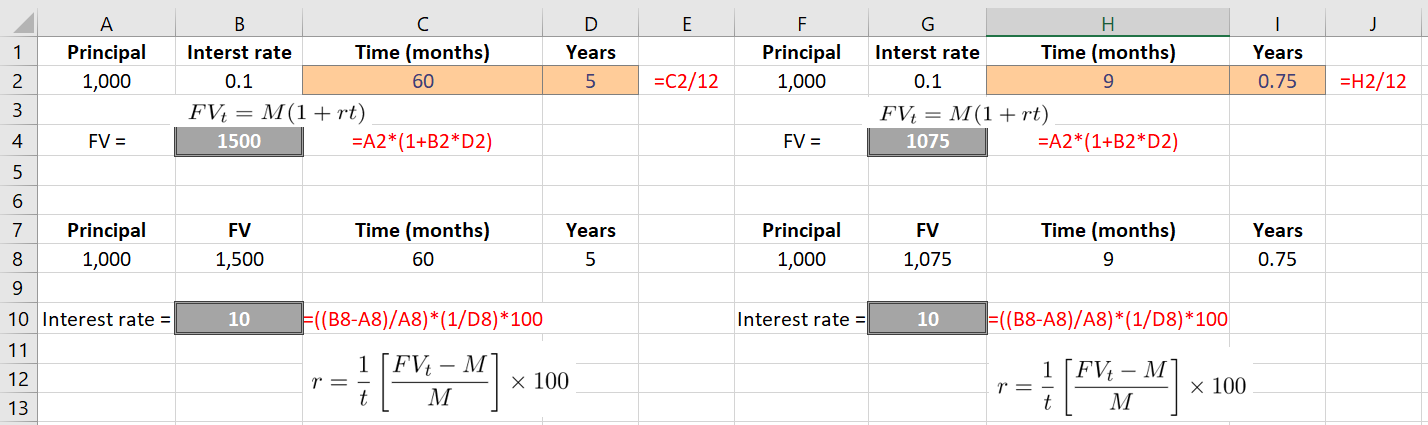
![\[FV_t= M(1+rt)\]](https://myriskbook.com/wp-content/ql-cache/quicklatex.com-9a01c2a63c5ec014e3012627c66b8f9f_l3.png "Rendered by QuickLaTeX.com")
![\[1+rt = {\frac{FV_t}{M}\]](https://myriskbook.com/wp-content/ql-cache/quicklatex.com-98f85882b25bb6f6f412d3e4cd7e79b8_l3.png "Rendered by QuickLaTeX.com")
![\[rt = {\frac{FV_t}{M} - 1\]](https://myriskbook.com/wp-content/ql-cache/quicklatex.com-543921c9a752c0bb3c6408fb8cc7094d_l3.png "Rendered by QuickLaTeX.com")
![\[r = \frac{1}{t}\left [\frac{FV_t}{M} - 1\right]\]](https://myriskbook.com/wp-content/ql-cache/quicklatex.com-64bd419aebf7e950c8c97607caad81e3_l3.png "Rendered by QuickLaTeX.com")
![\[r = \frac{1}{t}\left [\frac{FV_t-M}{M}\right]\]](https://myriskbook.com/wp-content/ql-cache/quicklatex.com-4d10f61717d6446bcf6ac701ac58e484_l3.png "Rendered by QuickLaTeX.com")
![\[r = \frac{1}{t}\left [\frac{FV_t-M}{M}\right]\times 100\]](https://myriskbook.com/wp-content/ql-cache/quicklatex.com-3890ac1d19f7d0fc1d97a0a70b47b239_l3.png "Rendered by QuickLaTeX.com")
![\[\frac{FV_t-M}{M}\]](https://myriskbook.com/wp-content/ql-cache/quicklatex.com-44d545a6d39b83ad8a6aa28d833b0937_l3.png "Rendered by QuickLaTeX.com")
![\[r = \frac{\text {Total interest}}{M \times t} \times 100\]](https://myriskbook.com/wp-content/ql-cache/quicklatex.com-56d271c10f5450f73de7634c23027461_l3.png "Rendered by QuickLaTeX.com")